Interactive Kronig-Penney Solver & E-k diagram plotter

Uploaded on: 4/7/2026

Completed

Overview & Installation

The Kronig-Penney equation provides the solution to one of the most fundamental problems in solid-state physics: the behavior of electrons in a periodic potential. The equation is derived from the time-independent Schrödinger equation and describes how electrons move through a crystal lattice. This simulator provides an interactive platform to explore the effects of various parameters (lattice parameters as well as temperature) on the solutions of the Kronig-Penney condition, which gives the allowed energy levels for any value of k

In order to use this simulator, go to the GitHub repository and download the code as a .zip file

Unzip the file and load navigate to its directory through your terminal

Python is required to run this simulator. First, Install the following Libraries

pip install numpy matplotlib

Then, run the following command to start the simulator

streamlit run app.py

Motivation

The primary motivation of building this project, was to build a tool that mapped various concepts such as reciprocal space, brillouin zones, allowed & forbidden energy bands, density of states and fermi-dirac distribution to a single interactive platform. Often, these concepts are taught together, and students are expected to understand them and link them together. Through this simulator, I aim to go one step further, and visualize the link between them through scientific computing in the form of this simulator.

As a beginner to computational physics & simulations, solving the kronig-penney equation, implementing E-k diagram based on its solutions and also implementing temperature dependent density of states & fermi-dirac function helped me develop a deeper understanding of the concepts used and also helped to develop functional and algorithm-based thinking to implement physical equations to computational methods.

Features & Functions

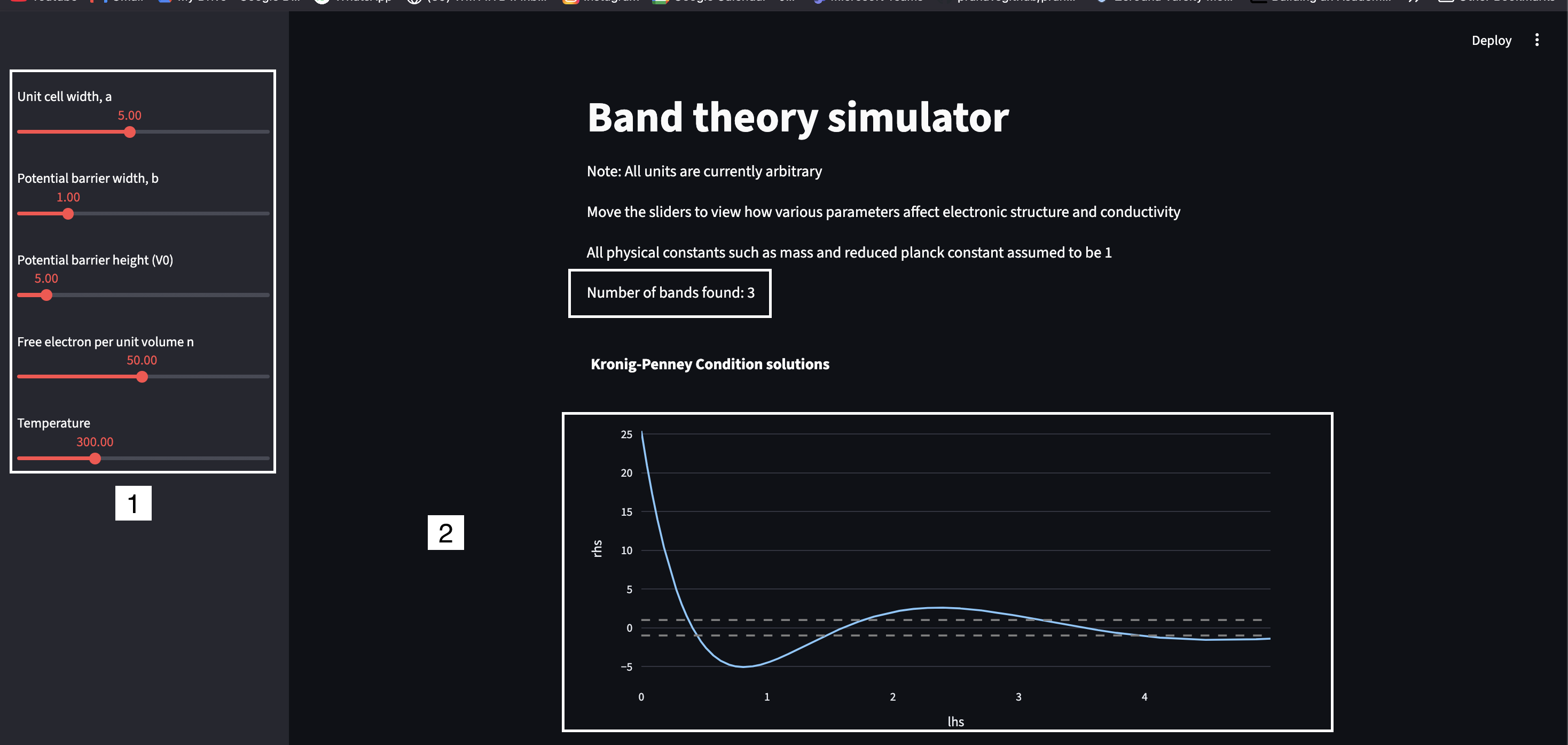
The simulator allows users to vary various parameters such as unit cell width (a), Potential barrier height(V) and potential barrier width(b), The values can be varied using the sidebar (1 in the picture) and the kronig-penney condition is graphically solved instantaneously in the graph shown in the picture (marked as 2)

The user can also vary the free electron density and Temperature, which are used for varying density of occupancy and fermi-dirac distribution

The number of bands indicates the number of solutions to the Kronig-Penney equation for the given values of a,b and V in arbitrary units

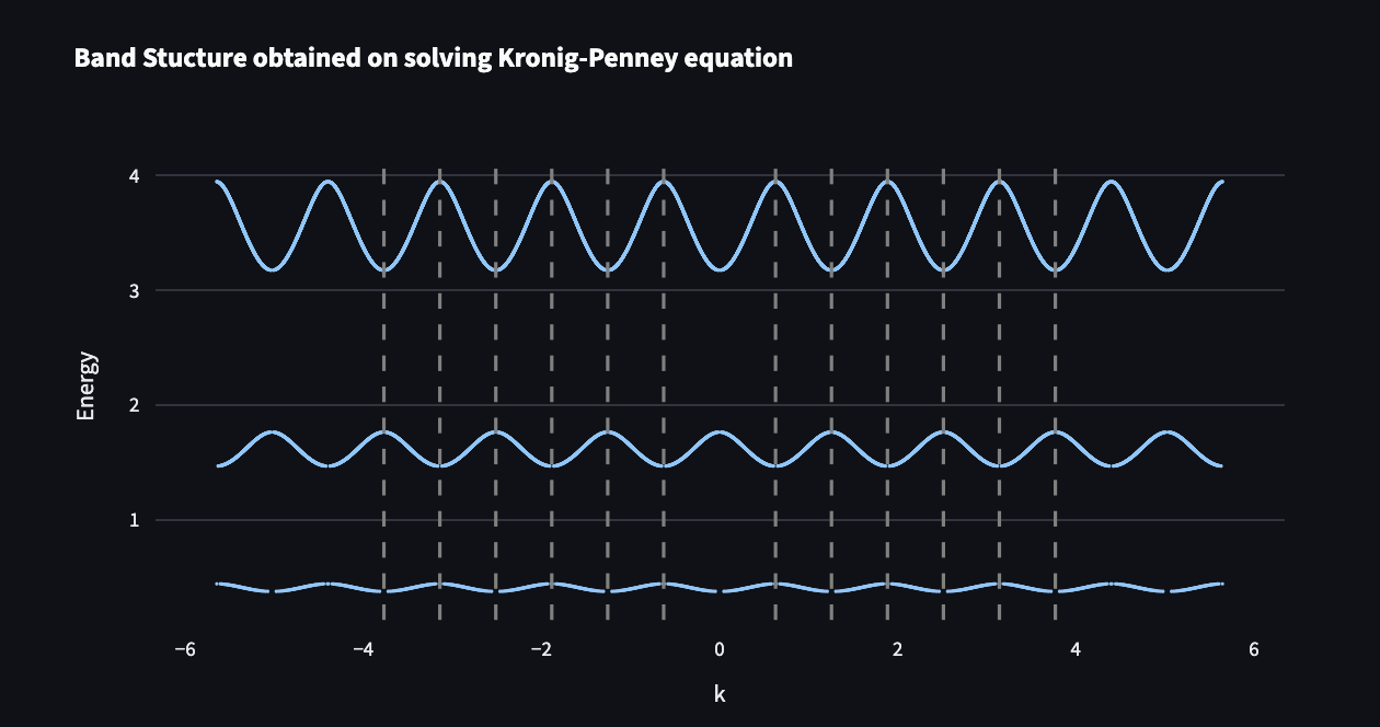
From the graphical solutions of the kronig-penney equation, an E-k diagram is generated, using the repeated k-space notation, which helps visualize the electronic band structure

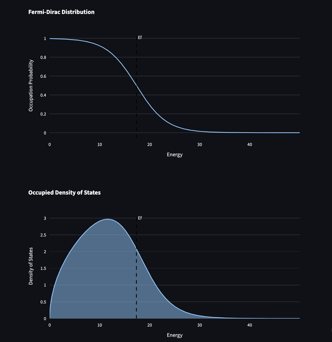
Further, electronic density of states is shown, however since factors like effective mass stay constant throughout this simple 1-D simulator, this remains constant for all values of a,b and V.

Fermi-dirac distribution has also been implemented as a function of temperature. Further, density of states is multiplied with fermi-dirac distribution to give the density of occupancy

Working of the Simulator

Allowed Energies Determination

At the heart of this simulator lies the kp_solver and allowed_regions functions, which calculate the graphical solutions to the kronig-penney equation

The code for the functions has been attached below:


def kp_solver(E, a, b, V0):
    if E <= 0 or E >= V0:
        return np.nan

    alpha = np.sqrt(V0 - E)
    beta = np.sqrt(E)

    const_term = (alpha**2 - beta**2) / (2 * alpha * beta)

    F = (
        const_term * np.sinh(alpha * b) * np.sin(beta * (a - b))
        + np.cosh(alpha * b) * np.cos(beta * (a - b))
    )

    return F


def allowed_regions(a, b, V0, points=20000):
    energies = np.linspace(1e-4, V0 - 1e-4, points)
    rhs = np.array([kp_solver(E, a, b, V0) for E in energies])
    allowed_bool = np.abs(rhs) <= 1

    return {
        "energy": energies,
        "rhs": rhs,
        "allowed_regions": allowed_bool,
    }

Standard Kronig-Penney Equation

\cos(ka)=\cos\!\big(\beta(a-b)\big)\cosh(\alpha b)+\frac{\alpha^2-\beta^2}{2\alpha\beta}\sin\!\big(\beta(a-b)\big)\sinh(\alpha b)

\alpha=\sqrt{\frac{2m(V_0-E)}{\hbar^2}},\qquad\beta=\sqrt{\frac{2mE}{\hbar^2}}

The function kp_solver defines the various parameters involved in the kronig-penney equation. It is purely a helper function which helps with the mathematical modelling of the kronig-penney equation. The inputs recieved are the energy(E), unit cell width(a), potential barrier width(b), and potential barrier height(V0). Physically impossible conditions are eliminated first and then the parameters alpha and beta in the standard kronig-penney equation are calculated. The constant term for the equation is then calculated and a single float value named 'F' is returned, which is the value of the right hand side of the kronig-penney equation for the given inputs.

The allowed_regions function then enforces the trignometric function condition i.e absolute value of cos(ka) is less than or equal to 1. The function works by generating an array of energy values with a linear difference between values with a user-defined number of points for accuracy, which is defaulted to 20,000. The E array is passed onto the kp_solver function which then calculates the value of the rhs. A boolean allowed_bool is used to designate which values of rhs are allowed for the given energy

The allowed_regions function returns a dictionary containing the array of energy values, calculated rhs values and a unique true/false value corresponding to each rhs and energy value, that indicates whether the value of rhs i.e the values of lattice parameter (a), potential barrier width (b) and potential barrier height (V0) for the given energy value is allowed or not. These allowed/forbidden regions are then used further for solving the lhs with the rhs and determining value of k corresponding to the allowed energies.

Graphical solutions plot

Using a simple matplotlib based plot, the values of rhs are plotted as a function of the energy values. The fact that absolute value of rhs cannot exceed 1 is depicted by the dotted lines. Also, the file kpsolver.py has been designed to be modular, and the user can choose to get detailed plots of rhs v/s energy itself by running the file in standalone mode.

Implementation of allowed Energies with k-space

The function band_compute in bandsolver.py is used for computing E v/s k relationships and the code for them is attached below

from kpsolver import *
def band_compute(a,b,V0,
                 points=5000, zones=4):
    kp_data = allowed_regions(a,b,V0, points)
    energies = kp_data["energy"]
    rhs = kp_data["rhs"]
    allowed = kp_data["allowed_regions"]
    allowed_E = energies[allowed]
    allowed_rhs = rhs[allowed]
    k_pos = np.arccos(allowed_rhs)/a
    k_dash = -k_pos
    G = 2 * np.pi / a
    k_all = []
    E_all = []
    for n in range(-zones, zones+1):
        shift = n*G
        k_all.extend(k_pos+shift)
        E_all.extend(allowed_E)
        k_all.extend(k_dash+shift)
        E_all.extend(allowed_E)

    return{"k_pos": k_pos  , "k_dash": k_dash, "energy":allowed_E, "k_all":k_all,
           "E_all":E_all, "G": G}

The function recieves input from allowed_energies and filters out the disallowed values, and also establishes the E-k relationship

Allowed arrays of E and rhs are generated based on the boolean values obtained from previous calculations, and finally, the lhs i.e cos(ka) is related with the rhs. Further, the function expands the array for a periodic lattice, using the reciprocal unit vector G and the number of zones to be plotted. The function returns a dictionary containing the allowed values of k and E, as well as the expanded arrays for plotting the E-k diagram.

For plotting the E-k diagram, the k_all array is used as x-axis and allowed_E is used as y axis

Fermi level determination

The Fermi level is a function of the number of free electrons in the system. In our case, the density of states is given simply as a function of the square root of Energy in 1-Dimensions as all the physical constants & scaling factors are taken as 1. The density of states is thus, constant for all values of n and T. The fermi-dirac distribution on the other hand is established as a function of the temperature.

By the conservation of mass, we get the simple relation

\int D(E)f(E,T)dE = N

An iterative approach is implemented to determine Fermi level. The function find_fermi_energy is attached below:

def find_fermi_energy(E, DOS, n, T):

    low = np.min(E)
    high = np.max(E)

    for _ in range(60):

        Ef = 0.5 * (low + high)

        f = fermi_function(E, Ef, T)

        electrons = np.trapezoid(DOS * f, E)

        if electrons < n:
            low = Ef
        else:
            high = Ef

    return Ef

The function uses binary sort along with trapezoidal rule of integration to determine fermi energy as a function of the total number of free electrons in the system

60 iterations of the binary sort algorithm are performed to converge on the Fermi energy. Initially, fermi energy is taken as average of extrema of parsed energy values. Trapezoidal rule is then used to integrate product of density of states and fermi-dirac distribution for each pair of consecutive energy values. The integral calculates the area under the curve for occupation of states. This is compared to total number of electrons and a decision for binary sort is taken.

Challenges faced

The first challenge I had faced with the project was choosing an approach to solve the kronig-penney equation and implement the E-k relationship. I had initially thought of using bloch-floquet boundary conditions to solve the equation and implement E-k relationship directly, but realized that it would be better to use the graphical solution approach, as the equation would be transcendental, and much harder to implement if solved directly.

The second, and perhaps the most significant challenge was implementing the graphical Kronig penney equation to establish E-k relationships, I wasn't sure on how allowed states could be implemented to pre-calculated energy values, especially since I only had a basic level of knowledge on array operations and functions. Using marker booleans to filter out allowed states was a simple and effective solution

The third issue I faced was in implementing an algorithm to determine fermi energy. Upon initial research, newton-rhapson method seemed to be suitable for finding a value of Ef that converged such that the integral of density of states and fermi-dirac distribution equaled the number of free electrons. However, I realized that this method would not be suitable for all cases as the derivative for the distribution of occupancy function has to be approximated, and caused failed convergence for certain values of n and T. I then implemented a binary sort algorithm to determine fermi energy, which although uses more iterations, converges for all values of n and T.

Improvements & Future project ideas

Based on additional knowledge I have gained since this project, I think the following ideas would be suitable for future projects

Expansion of the model to 3-D k-space
Implementation of real-life E-k relationships for basic semiconductors such as Si, Ge, GaAs
Incorporation of doping and ionization of dopants & carrier concentration simulation
Mathematical analysis of non-degeneracy & boltzmann approximation